Using the Query Table Data Construct

< Previous		Next >

Associating with a Query Operator

A Query Table data construct is always associated with one or more Query operators, which are described in Using the Query Operator.

The Query Table data construct does not have input and output ports, and the flow of tuples in your application does not typically flow through a Query Table. Instead, each Query Table data construct must be associated with at least one Query operator. Use the Query operator to read from, write to, delete from, or update your Query Table.

To draw an association arc between a Query Table data construct and a Query operator:

Select the gray square on the bottom port of the Query operator, and hold down the mouse button.
Drag the mouse pointer to the gray square at the top of the Query Table data construct.
Release the mouse button.

If you mark a Query Table as shared, then outer modules can run queries on the shared Query Table in an inner module and vice versa. In this case, you draw an association arc between a Query operator and the Module Reference, both in the outer module.

Affected Components Link

At the top of the Properties view for a Query Table data construct, there is an Affected Components link. Click this link to display a pop-up window that lists the Query operators in the current module that are associated with the selected Query Table. Click anywhere outside the pop-up to close the pop-up.

The following example shows an Affected Components pop-up window that shows the Query operators associated with the Nasdaq100Table Query Table in the Query.sbapp sample application, which is a member of the operator sample group shipped with StreamBase.

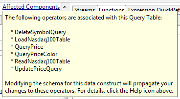
The EventFlow diagram for the sample application looks like this:

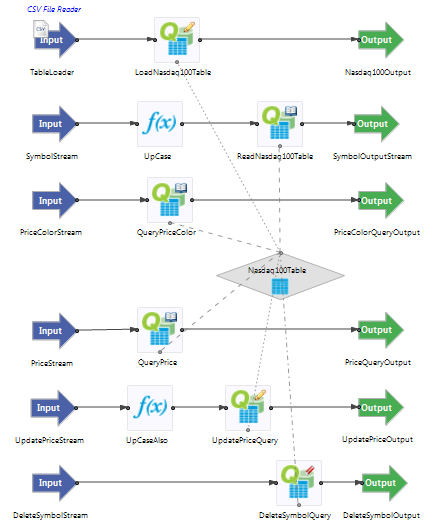
Notice that the Nasdaq100Table Query Table is referenced by six Query operators, two of which write into the table, three of which read from the table, and one that deletes rows in the table.

Properties: General Tab

Name: Use this required field to specify or change the name of this instance of this component, which must be unique in the current EventFlow module. The name must contain only alphabetic characters, numbers, and underscores, and no hyphens or other special characters. The first character must be alphabetic or an underscore.

Description: Optionally enter text to briefly describe the component's purpose and function. In the EventFlow canvas, you can see the description by pressing Ctrl while the component's tooltip is displayed.

Properties: Table Settings Tab

Use the Table Settings tab to specify this Query Table's type and behavior. The following image shows the tab with all default values:

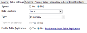
The following table describes the Table Settings tab options.

Property	Default	Description
Shared	No	Controls the visibility of this Query Table across application modules. Use this setting to mark the data in this Query Table as accessible from outside the module that defines it. Setting Shared to No restricts this Query Table's visibility to the module that defines this Query Table. This is the default setting. Setting Shared to Yes marks this Query Table in the current module as accessible to a Query operator in a separate module or container. When a Module Reference refers to a module that contains a Shared Query Table, its icon displays a gray data port on its top edge, similar to the data port on top of a Query Table icon. You can connect a Query operator in the separate module to the shared table by means of this data port. Important StreamBase does not support exporting a Query Table from a Module Reference with a multiplicity setting greater than 1. See Concurrency Options for details. When you define a Query Table with a table schema, you must still specify the memory versus disk table Type, the Access Label, and other settings on the Table Settings tab for this table.
Enable Data Stream port	No	When you select Yes, the Query Table's icon gains a Delta Stream port on its right vertex. An event tuple is emitted on the Delta Stream port for every change to the table's contents.
Data Location	Local	Specifies where data for this Query Table can be found. Use this setting to access a table that is not in the current module. The options for Data Location are: Local Indicates that this table is defined locally by this Query Table data construct. The table can be accessed by other modules if Shared is set to Yes. Defined by Calling Module Indicates that this table is defined in a module that incorporates the current one. No additional Table Settings options are available for tables defined in other modules. Defined by Connection Path Indicates that this table is defined in another module, possibly in a separate container. This option is similar to the Defined by Calling Module option, except that the module containing the Query Table need not contain the current module; instead, it may exist in a separate container intended to be accessed at run time. When you select this option, a Connection Path field displays below the Data Location menu. You must enter a path to the container in this field. The general notation for paths is: `container.{module.module...}.table-name` The path to the shared Query Table, always specifying the container name, even if it is `default`. For example, if a Query Table named `PriceTable` is in `Main.sbapp`, which it the top-level EventFlow module for an application, use the path `default.PriceTable`. If `PriceTable` is in `CalculatePrices.sbapp`, which is called through a module reference named `calculate` in `Main.sbapp`, then use the path `default.calculate.PriceTable`. Use the sbc command `sbc list -ac containers tables` on your running application to obtain a list of Query Table path names. The following is the result of that command run against the Cross Container Table sample included with StreamBase, when started from its deployment file: container default container reader container system container writer table default.LocalTable table reader.TableConnected table writer.TableConnected A Query Table defined this way is an abstract pointer to an actual Query Table in another module, and is referred to as a Placeholder Query Table. A module that contains a Placeholder Query Table can pass typechecking without access to the actual Query Table.
Type	In memory	Specifies the persistence of this Query Table. The options are: In memory In memory Query Tables are fast and efficient, but their data is not persisted and is not available after the hosting StreamBase Server shuts down. On disk Data in this Query Table is stored and is available for the application the next time the server starts. When using this option, you can designate a data directory to contain the persisted Query Table data, as described in Setup For On-Disk Query Tables, or you can accept the default location. The On disk option is only available only if your StreamBase license enables it. You can also enter a parameter, such as `${tabletype}`, in the Type control. The module that contains this table must contain or be passed a parameter having the name you specify. The parameter value must be either `disk` or `memory`.
Truncate on startup	(dimmed)	This setting applies only to On disk Query Tables. If set to `Yes`, then on startup of the containing StreamBase Server: If the table already exists, all of its records are deleted. That is, the table is initialized. If the table does not exist, it is created. If set to `No`, then on server startup: If the table already exists in the specified data directory, it is opened and any records in it remain as they were. If the table does not exist, it is created. This setting can interact with settings on the Initial Contents tab.
Enable Table Replication	No	Selecting Yes causes the servers in a high-availability design pattern to maintain the state of the tables on each server so that either can become the leader in case of failover to the other. When using this option, you must also configure the parameters in the `<high-availability>` section of the server configuration file for each server in a high-availability cluster. See Replication of Query Tables for further instructions.

The EventFlow canvas icons for Shared and Placeholder Query Tables are overlaid with decorations to distinguish them from concrete, private Query Tables. When a table is shared, the table within the has a green dot overlay in its lower right corner. If the table is not local to the module, it has a blue triangle overlay in its lower left corner.

In addition, a Query Table that implements a StreamBase interface is shown with a boxed uppercase I in the lower right corner of the icon's tile:

Properties: Schema Tab

The following table describes the Schema tab options.

Property	Default	Description
Table Schema	<Private Table Schema>	Either choose an existing table schema or define a private table schema for this table. The default setting enables you to define a schema in the grid below. You must also define your table's indexes using the Primary Index and Secondary Indices tabs. Private schema definitions are local to this Query Table and to the containing module. You can instead select the name of a previously-defined table schema from the drop-down list. The schema and index definitions for this Query Table are taken from the specified table schema. As a table schema defines indexes, you cannot change them using the Primary Index and Secondary Indices tabs. 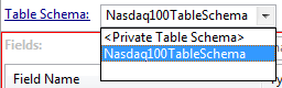The Table Schema drop-down list only lists table schema names if the containing module defines or imports at least one table schema. Table schemas are discussed further in Using Table Schemas. When you define a Query Table with a table schema, you must still specify the other settings (for example, memory versus disk table) on the Table Settings tab for this table.
Fields	Inherited or empty	Unless you have specified a <private table schema> for this table, the Fields drop-down is dimmed, and the fields of the schema grid are populated by the table schema and are non-editable. When enabled, the Fields drop-down lets you choose from available named schemas. To configure a local schema, set the Fields drop-down to <private schema>. Enter a private schema for this table and then define indices for it, as described below.

Property

Default

Description

Table Schema

Either choose an existing table schema or define a private table schema for this table. The default setting enables you to define a schema in the grid below. You must also define your table's indexes using the Primary Index and Secondary Indices tabs. Private schema definitions are local to this Query Table and to the containing module.

You can instead select the name of a previously-defined table schema from the drop-down list. The schema and index definitions for this Query Table are taken from the specified table schema. As a table schema defines indexes, you cannot change them using the Primary Index and Secondary Indices tabs.

The Table Schema drop-down list only lists table schema names if the containing module defines or imports at least one table schema. Table schemas are discussed further in Using Table Schemas.

When you define a Query Table with a table schema, you must still specify the other settings (for example, memory versus disk table) on the Table Settings tab for this table.

Fields

Inherited or empty

Unless you have specified a <private table schema> for this table, the Fields drop-down is dimmed, and the fields of the schema grid are populated by the table schema and are non-editable. When enabled, the Fields drop-down lets you choose from available named schemas. To configure a local schema, set the Fields drop-down to <private schema>. Enter a private schema for this table and then define indices for it, as described below.

Use the Schema tab to select a previously defined table schema, which replaces both schema and index settings for the entire table. If you specified an existing Table Schema, then the Fields drop-down is disabled. In this case, the specified table schema is responsible for providing this Query Table's schema. If you specify no Table Schema, you can select a previously-defined named schema, which provides only the schema definition, leaving the index settings to you.

If the Table Schema drop-down names an existing schema, then its fields are populated in the grid beneath it. You can select and copy the fields but cannot edit them. If you set the drop-down to <Private Table Schema>, then you can define the schema for this Query Table, as follows:

Type text into the optional Schema Description field at the bottom of the Schema tab to document your schema.

Select <Private Schema> in the lower drop-down list. (The drop-down list provides no other choices unless you have defined or imported at least one named schema for the current module.)

Private Schema

Populate the schema fields using one of these methods:

Define the schema's fields manually, using the Add button to add a row for each schema field. You must enter values for the Field Name and Type cells; the Description cell is optional. For example:

Field Name	Type	Description
symbol	string	Stock symbol
quantity	int	Number of shares

Field names must follow the StreamBase identifier naming rules. The data type must be one of the supported StreamBase data types, including, for tuple fields, the identifier of a named schema and, for override fields, the data type name of a defined capture field.

Add and extend a parent schema. Use the Add button's Add Parent Schema option to select a parent schema, then optionally add local fields that extend the parent schema. If the parent schema includes a capture field used as an abstract placeholder, you can override that field with an identically named concrete field. Schemas must be defined in dependency order. If a schema is used before it is defined, an error results.
Copy an existing schema whose fields are appropriate for this component. To reuse an existing schema, click the Copy Schema button. (You may be prompted to save the current module before continuing.)

In the Copy Schema dialog, select the schema of interest as described in Copying Schemas. Click OK when ready, and the selected schema fields are loaded into the schema grid. Remember that this is a local copy and any changes you make here do not affect the original schema that you copied.

The existing schema can be from a system stream, or from any named or unnamed schema defined in the current module or in another application in your workspace. You can also select a CSV text file and populate a schema with its column headers. Studio will attempt to infer data types from the first few rows of values, and you can override the types it identifies. Currently, auto-detection of int, double, boolean, string, timestamp and tuples are supported, but not lists or functions. When indicating tuples, the CSV header must identify subtuples with dot notation, for example as stock.symbol, stock.price.

Use the Remove, Move Up, and Move Down buttons to edit and order your schema fields.

Named Schema

Use the drop-down list to select the name of a named schema previously defined in or imported into this module. The drop-down list is empty unless you have defined or imported at least one named schema for the current module.

When you select a named schema, its fields are loaded into the schema grid, overriding any schema fields already present. Once you import a named schema, the schema grid is dimmed and can no longer be edited. To restore the ability to edit the schema grid, re-select Private Schema from the drop-down list.

Properties: Primary Index Tab

If you specified the name of a table schema in the Table Schema drop-down in the Schema tab, the Primary Index tab shows the primary index field or fields defined in the table schema. You cannot edit the index fields.

If you specified <Private Table Schema> the name of a table schema in the Table Schema drop-down, then you must use the Primary Index tab to define the primary index field for this Query Table.

Query Tables must have a primary index to be valid. Use the Primary Index tab to select a schema field or fields that will be used to look up values in the Query Table. Usually, the primary index field or fields are those that the associated Query operators will use most often. For example, in a table that stores stock trade information, the field that holds the stock symbol is likely to be queried often.

In the Available Fields list, double-click each field that you want to add to the index (or select a field and click the right arrow button). If a Query Table's schema includes fields of type list or tuple, you can use a subfield as the field specification.

Tip

A timestamp field is usually a poor choice for a Query Table primary index, because multiple input tuples can have identical timestamps, and primary index values must be unique. Instead of a timestamp, consider using a Sequence operator to generate unique IDs. See the Sequence operator sample for a simple illustration of this technique.

In the Available Fields list, double-click each field that you want to add to the index (or select a field and click the right arrow button).

Use the Index Type control to select how keys are indexed for table read operations:

Unordered, no ranges (hash):: Keys are unsorted, and they are evenly distributed (hashed) across the index. A hash index is used for accessing keys based on equality, and are generally best for doing simple lookups.
Ordered, with ranges (btree): Keys are sorted. A btree index is used when output ordering and range queries are desired. Note that the sort depends on the order of the fields in the index keys.

The relative performance of hash and btree methods varies depending on many factors, including the distribution of keys in your dataset. If you are in doubt, try both methods to determine which produces the fastest lookup times for associated Query operators. Also remember that StreamBase Studio allows you to specify a key range and sort order in an associated Query operator when you use a btree ordered index, but not when using hashed access.

Properties: Secondary Indices Tab

If you specified the name of a table schema in the Schema tab, then entries in the Secondary Indices tab are pre-set by the table schema, and you cannot edit or add to them.

When the Table Schema is set to <Private Table Schema>, you can use the Secondary Indices tab to define one or more secondary index fields for this Query Table.

Secondary indexes specify a field or set of fields that are used to look up values in the Query Table. Secondary indexes are optional; if used, no secondary index field can be the same as the primary index field. If a Query Table's schema includes fields of type list or tuple, you can use a subfield as the field specification.

For each secondary index:

Click Add to display the Edit Secondary Index dialog.
In the Available Fields list, double-click each field that you want to add to the index.
Click the Add to Index List button.

Tip

Timestamp fields are usually poor choices for a Query Table secondary index, because multiple input tuples can have identical timestamps. Instead of a timestamp, consider using a Sequence operator to generate unique IDs. See the Sequence operator sample for a simple illustration of this technique.

Fields are indexed using the btree method by default. Just as with primary indexes, you can also use the hash method. To change the index type, select Ordered or Unordered at the bottom of the Edit Secondary Index dialog. You can intermix hash and btree indexes in the same Query Table. For example, the primary index could be hash and a secondary index could be btree.

Secondary indexes make write and delete operations slower, because each secondary index in the Query Table must be updated with every change to the Query Table.

You can use an expression as part of specifying the field or fields that comprise a secondary index for a Query Table. The expression must be statically resolvable, and must contain the name of at least one field in the Query Table's schema. A sample in the Operator Sample Group illustrates this feature.

Properties: Initial Contents Tab

Use the Initial Contents tab to specify the starting point contents of this Query Table at module startup. Query Tables that load initial contents at startup show a red asterisk overlay:

The options on this tab are only available when you have specified Local in the Data Location drop-down on the Table Settings tab.

Query Tables running in heap can always have their initial contents loaded with this feature, because such tables are always initialized at the start or restart of the containing module.

However, using this feature with an on-disk Query Table requires careful consideration of the consequences:

The loading of initial contents occurs with a Write-Update operation based on a primary key match. This means that:
- Any matching rows in the on-disk table are overwritten with the initial contents version of that row.
- Any matching row that was deleted in the last run of the module (whether that row was previously loaded initially or inserted during that run) is restored to its initial contents state.
- Let's say you load 100 rows from an initial contents file, and then add 25 more rows, update 10 rows, and delete 5 rows. Restarting the containing module does not overwrite the first 100 rows. Instead, it looks for 100 primary key matches anywhere in the table's current 120 rows and overwrites matching rows with initial contents data — whether or not those matching rows were updated in the previous run. Some deleted rows may be restored. In summary, on module restart, the Query Table contains 120 to 125 rows, depending on whether any deleted initial rows were restored. However, the table does not have the same contents as when the module last ended.
If your goal is to truly wipe the Query Table clean and reload it with the same initial on-disk contents every time, then combine this Initial rows feature with the Table Settings tab's Truncate on startup setting.

This tab's options are:

Be empty

The default option is to not load the Query Table at module start time. Select this option under the following circumstances:

If you want this table to start as a clean slate at module start time, to be populated by upstream operators as the containing module runs.
If this table will be loaded at start time by an external operator such as a CSV File Reader adapter.

Load initial rows from a resource file, CSV

Select a resource file in CSV format, which must already exist on this module's resource search path. The initial loader's CSV reading capabilities are a strict subset of the features available in the CSV File Reader adapter and the Feed Simulation CSV Data File Option. The initial loader CSV file has the following restrictions:

You must use commas as the field separator.
The file's columns must exactly match the schema of the Query Table in number and data type for each field.
The null keyword is not accepted, but you can specify empty fields with a pair of adjacent quotes: ""
Date format strings are not interpreted as timestamp fields. Specify the exact literal time instead.
Specify the fields of the tuple data type as a comma-separated list between double quotes. For example, for the schema (a int, b (b1 int, b2 int), c string), enter CSV rows like the following:
```
3, "10, 20", alpha
4, "20, 30", beta
```

If the CSV file to be loaded contains a header row, select the Skip header row check box, otherwise leave it unchecked.

The operators sample group includes a CSV file, ResourceFiles/NASDAQ100.csv, in the correct format for use as an initial table loader. Use this file with the Query.sbapp module, replacing the CSV File Reader adapter currently in place.

Load initial rows from a resource file, TSV

TSV stands for tab-separated values. TSV files follow the same rules as CSV files, but use a hard tab character as the field separator instead of a comma. This includes using a tab character between the subfields of a tuple field.

Load initial rows from a resource file, JSON

Select a file from this module's resource search path, containing one or more JSON objects, each on its own row. JSON objects are defined on json.org as a set of comma-separated field-value pairs, with pairs separated by a colon, and with the entire object surrounded by braces. Strings in JSON are surrounded by double quotes. There is no header row in JSON format.

For example, following are the first two rows of the NASDAQ100.csv file expressed in JSON object format, with truncated Description fields for readability. The two lines are shown here on four lines for publication clarity:

{ Name:"Activision Blizzard, Inc",Symbol:"ATVI",Price:12.71,Color:"red",
      Description:"Activision Blizzard ..."}
{ Name:"Adobe Systems Incorporated",Symbol:"ADBE",Price:28.43,Color:"yellow",
      Description:"Founded in 1982, ..."}

To specify the subfields of a field of type tuple in JSON object format, use a nested pair of braces. For example, for the schema (a int, b (b1 int, b2 int), c string), enter JSON rows like the following.

{a: 3, b: {b1: 10, b2: 20}, c: "alpha"}
{a: 4, b: {b1: 20, b2: 30}, c: "beta"}

You can also use JSON array format as defined on json.org, like this example:

[3, [10, 20], "alpha"]
[4, [20, 30], "beta"]

In both JSON object and array formats, white space is ignored, but you must use commas to separate tuple fields.

Load initial rows from the text below, CSV, TSV, or JSON

Select this option and type one or more rows of data in CSV, TSV, or JSON format, using the same rules as for the files described above.

If you provide a CSV, TSV, or JSON loader file whose fields fail to match the table's schema, or if you type mismatched rows in the Initial Contents tab, a typechecking error is shown in associated Query operators as well as in the Properties view for the Query Table itself.

Null Values

If the key field for a tuple record being written to a Query Table is null, the tuple is stored. In a Query Table with a sorted (btree) index, the null-keyed stored records are evaluated as less (in value) than other non-null records. On a subsequent read (lookup) operation, the null-keyed tuples can be located. For more information, see Using Nulls.